Graduate Research Updated: December 05, 2006
University of Washington with the College of Forest Resources
Generating Stream Maps Using LiDAR Derived Digital Elevation Models
Remotely Sensing Forest Cover for Various Counties
Generating Stream Maps Using LiDAR Derived Digital Elevation Models and 10-m USGS DEM
1. INTRODUCTION
1.1 Overview
Streams are one of
the most valuable public resources in the State of
However, new mapping technology provides the potential of developing improved stream data from more detailed surface topology. LiDAR (Light Detection And Ranging) data which creates sub meter topography maps (Appendix A) is one technology that promises to provide increased resolution in digital surface detail compared with the typical 10 meter topographic maps and could lead to more precise and accurate maps of stream networks. Preliminary analyses showed that using LiDAR data located more actual stream channels and placed streams in their topographically correct position (Schiess and Tryall, 2002). This ability to generate accurate stream locations and physical attributes using LiDAR will allow long-term sustainable harvest volume calculations to be more reliable.
In order to properly map the physical extent of channels in a watershed, the difference between processes on hillslopes and in channels must be determined (Tarboton 2003). This difference becomes apparent when calculating how water collects on a landscape in a given dataset with flow direction of the water known.
In
channels flow is concentrated. The
drainage area, A, (in m2) contributing to each point in a channel may
be quantified. On hillslopes flow
is dispersed. The "area" draining
to a point is zero because the width of a flow path to a point disappears. On hillslopes flow and drainage area
need to be characterized per unit width (m3/s/m = m2/s for
flow). The specific catchment area,
a, is defined as the upslope drainage area per unit contour width, b, (a = A/b)
(
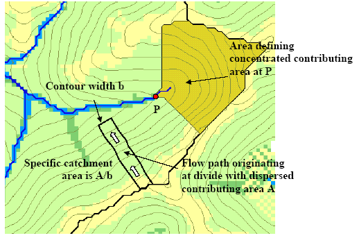
Figure 1. Definitions of concentrated and dispersed contributing area and specific catchment area (Tarboton 2003).
LiDAR can place these physical attributes in their topographically correct position. However, locating point ‘P’ (Figure 1), the perennial initiation point (PIP), becomes a challenge due to it being dependent on the catchment area which fluctuates based on geology, climate, precipitation, and other attributes.
1.2 Previous Studies and Background Review
Various
hydrological models such as Simulator for Water Resources in Rural Basins
(SWRRB), Environmental Policy Integrated Climate (
Figure 2
demonstrates topographic error in the Washington

Figure 2.
Figure 3 shows the contours generated from a standard 10-m DEM overlaid on a 2m LiDAR-derived hillshade model with slope classes from the LiDAR derived DEM. Downhill is toward the upper right. LiDAR topography provided a realistic and detailed topography. Photogrammetricly produced contour lines captured the general shape of the landscape; however, complex features such as incised streams, draws, abandoned road beds and sharp ridges were not recognized (Schiess and Krogstad, 2003). The contour lines also do not follow the stream channel accurately.
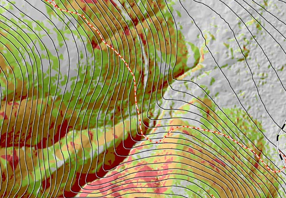
Figure 3. A Lidar-hillshade derived from 2m grids
versus the contours, derived from
The advantage of LiDAR digital data over conventional photogrammetry is improved mapping in obscured areas. A LiDAR bare ground surface model containing only elevations can be obtained after filtering out the trees and buildings in the dataset. The digital data then can be used in a variety of ways including: digital terrain model for use in generating contours, 3D terrain views, fault locations, steep slopes, critical areas, and stream and drainage basin delineation (North Carolina 2003).
One attempt to use LiDAR data to generate stream channels at the College of
Forest Resources, University of Washington was on the South Tyee Planning Study
in 2002 (Schiess and Tryall, 2002).
The stream layer was produced by the “flowaccumulation” command in GRID
and a uniform buffer was added (Figure 4).
The stream layer could be adjusted by changing the contributing cells to
the stream, which made it possible to duplicate conditions observed in the
field. The contributing cell size
was adjusted to a slightly higher level in order to include areas that may not
have contained water at the time.
It should be noted that while the

Figure 4. Stream
layer produced from flow accumulation model in ArcGIS with 75-ft buffer using
LiDAR at left compared to
There were many discrepancies in comparing the LiDAR “flowaccumulation”
streams with a
Table 1. Area Covered by Buffers in
With better field reconnaissance and appropriate buffer widths a more accurate stream layer could be produced. However, the LiDAR stream data provided a better input for the preliminary planning process than the 7.5 minute stream data (Schiess and Tryall, 2002).
1.3 Current Stream Data
The current stream
data was created by the
The Water Type process occurred during a
time of significant and rapid improvement in technical information and software
tools. As a result of the extensive
fish surveys being performed, abundant field survey information was available
for many areas of the state.
Advances in
The physical attributes for the Water Typing model were based on a USGS 10-DEM. Using this DEM, physical barriers such as waterfalls and downstream gradient could be overlooked due to the low resolution. Furthermore stream channels predicted using aerial photos under and over estimate stream locations due to visibility. At times, the channels were topographically off from the actual location of those channels (Schiess and Tryall, 2002).
The current
- type 1, 2, and 3 --------- Fish bearing waters
- type 4 and 5------------- Non-fish bearing waters
- type 9-------------------- Untyped, unknown
Types 1-4 are considered perennial and type 5 and 9 are seasonal. The second code either describes streams as fish-bearing or non-fish bearing waters. This code was derived from the Cooperative Monitoring, Evaluation, and Research group (CMER) using the CMER Model as described in the Method / Model Development section. The same channel network is used for both code systems.
1.4 Research Objectives
The goal of this project is to determine if LiDAR would improve stream network classification. Therefore the following questions needed to be answered:
- Does an increase in resolution improve stream channel determination?
- Can stream types be determined more accurately using LiDAR datasets?
- Can a new algorithm be developed for identifying perennial streams?
To verify that the increased LiDAR resolution improves stream modeling, different hydrologic models were tested using a 10 meter USGS and several LiDAR DEMs at various resolutions. D8, D-Infinity, Multiple Flow, and DEMON were the model algorithms used (refer to section 2.5 Flow Direction Methods Utilized). Once the models were used and data was generated from the model, field verification was carried out to verify the accuracy of the predicted stream channels.
2. METHODS / MODEL DEVELOPMENT
Flow direction algorithms for locating stream channels were used on various
resolutions and correlated with field data. This was completed to establish which
flow direction technique worked best with LiDAR data. For stream typing, the Cooperative
Monitoring, Evaluation, and Research group (CMER) from the Washington State
Department of Natural Resources (
Three models needed to be developed in order to decide if resolution has an effect on stream channel determinations and if stream types could be determined more accurately by LiDAR. The first model is the generation of the stream network from LiDAR DEM. The second is a water-typing model to determine the end of fish point (EOFP) from the generated stream network and the third is the perennial initiation point (PIP) model.
2.1 Site Description
The
North fork of the Mineral Creek Watershed in the
Figure 5. The North fork of the Mineral Creek
Watershed in the
The mean annual
rainfall in this area ranges from 2007 to 2210 mm (Daly et al. 2000) with an
altitude range of 500 to 1600 m.
Forest cover is dominated by Douglas Fir (Pseudotsuga menziesii) with
Western Larch (Larix occidentalis), Red Alder (Alnus rubra), Big Leaf Maple
(Acer macrophyllum), Western Hemlock (Tsuga heterophylla), White Fir (Abies
concolor), and Black Cottonwood (Populus trichocarpa) throughout. The majority of the region’s soils
belong to the Bellicum, Cattcreek, and Cotteral soil series (Soil Survey Staff,
1998). The upper part of the
profile has a cindery texture from the pumice and volcanic ash aerially
deposited from
2.2 Stream Model
The type of streams that were modeled included all segments of natural waters within the bankfull widths of defined channels which are either perennial streams (waters that do not go dry any time of a year of normal rainfall) or were physically connected by an above-ground channel system to downstream waters. In extracting networks from DEM’s, Tarboton et al. (1991) suggest that the network extraction should have properties traditionally ascribed to channel networks and have as high resolution as possible. A LiDAR-generated DEM provides this high resolution and the physical properties, such as channel depth and slope, associated with a stream network.
2.3 Water-Typing Models
Two preexisting logistic regression models were used to identify potential fish habitat. The CMER Model takes into account several physical attributes while the Gradient Model focuses on the gradient of the landscape. LiDAR DEM data was used to generate the attributes needed to apply these models.
2.3.1
CMER Model The CMER Model was used to identify potential fish habitat. Based on previous research, this
habitat-based, water-typing model was developed using logistic regression
analysis and
The
fish absent | fish present (FAFP) data used to estimate the logistic regression
models were generated from 4,052 end-of-fish points (EOFP) placed on a
Washington Dept. of Natural Resources (
1. Basin size (number of acres in surrounding basin that drain through a point),
2. Elevation in feet (based on 10-m DEM network),
3. Downstream gradient which is the average gradient measured over 100-m downstream of the point (calculated from 10-m DEM network elevation information), and
4. Precipitation in
inches (
These four physical attributes associated with each EOFP point were the variables available for the logistic regression model building process.
Equation
1 is the response function where
![]() is the estimated
probability of fish presence.
is the estimated
probability of fish presence.
(1)
![]()
Equation 2 is the linear model where the variables are described in Table 2 (Conrad et al., 2003).
(2)
![]() = -7.717073 + (0.020166 * (PRECIP)) + (3.793994 *
(Log10(BASIZE))) –
= -7.717073 + (0.020166 * (PRECIP)) + (3.793994 *
(Log10(BASIZE))) –
(0.062949 * (DNGRD)) - (0.110926 * (ELEV / 100))
The CMER Water-Typing Model was applied to the LiDAR DEM in the same manner it was applied to the 10m DEM. Downstream gradient (DNGRD), Elevation (ELEV), and Basin Size (BASIZE) were determined by LiDAR using the LiDAR-derived stream network and elevation model. Table 2 provides the results of the logistic regression model (Conrad et al., 2003).
Table 2. Summary of the final logistic regression model coefficients, standard errors, significance of the coefficients, and 95% confidence intervals for the exponential
of the coefficients. (Conrad et al., 2003)
2.3.2 Gradient Model This model’s objective was to identify the
physical constraints and stream characteristics at the upstream limits of trout
distribution (Latterell et al., 2003).
Logistic regression was used to model the likelihood of trout presence in
a 100-m stream reach as a function of physical stream attributes using sites
described in Latterell et al. (2003) sites. The regression provided a probabilistic
prediction of trout presence because the dependent variable was binomial (trout
presence or absence). Further, this
technique does not assume normality, equal variances, or a linear response. Equation (1) from above is the response
function used for this model with
![]() as the linear
model, which is
as the linear
model, which is
(3)
![]()
where B1 is the Gradient Coefficient at -0.209 and B0 is the Model Constant
at 2.765. Logistic regression
calculates the probability of success identified as (i.e., trout presence,
![]()
![]() 0.50) over the
probability of failure (i.e., trout absence,
0.50) over the
probability of failure (i.e., trout absence,
![]() < 0.50).
< 0.50).
2.4 PIP Model
The
perennial initiation point (PIP) is the point where perennial flow begins on a
Type 4 Water. Type 4 Water means
all segments of natural waters within the bankfull width of defined channels
that are perennial non-fish habitat streams. The model for PIP was developed in a
Perennial initiation point standard is defined in
The PIP Model was
based on the techniques described in Conrad et al., (2003) except the logistic
regression was used to identifying where perennial flow begins and where it ends
instead of fish present. Stream
head data locations were collected in the field for 5 sub-basins within a
selected site. Points were
generated 15 meters upstream and downstream of the stream head in
1. Basin size – Using SAGA (System for Automated Geoscientific Analyses, a GIS system) (Appendix F) the algorithms described in the Stream Model section were utilized.
2.
Downstream gradient - Using the 2-m LiDAR DEM, focalmin was used in ArcMap
DG = float([2m DEM] – focalmin([2m DEM], circle, 50) / 328 * 100%
50 is 100 meters in mapping units for 2m grid cell size and 328 is 100 meters in ft.
3. Forest
Density - A spatial tree list was created using LiDAR by
CR = (H + .223) / 4.4
where CR is crown radius and H is height (Oladi 2001). A crown cover layer was created by buffering each point using the size of the crown radius and converting the resulting polygon coverage to a grid. Individual tree crown density was determined by taking an 11-m buffer around the tree point and dividing the area of the crown within the buffer by the area of the buffer.
4. Slope (calculated from 2m LiDAR DEM network elevation information in percent with ArcMap (%slope = 100 * Tan (∆y/∆x))),
5. Elevation in feet (LiDAR bare earth DEM),
6. Precipitation in
inches (
7. Site Class
(Downloaded from Washington
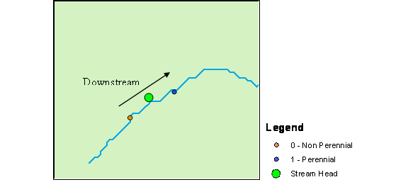
Figure 6. Plan view at a stream channel showing points generated 15 meters upstream and downstream of the stream head with physical attributes associated with the head. This is to produce a binomial linear regression model identifying perennial and non-perennial parts of a stream network.
The points upstream represented non-perennial flow as the points downstream represented perennial flow. Using binary logistic regression and setting 0 for non-perennial and 1 for perennial, the physical attributes associated with each point were used to develop Equation 1 from above and equation 4.
(4)
![]() =
b0+b1xi1+b2xi2+...+bpxip
=
b0+b1xi1+b2xi2+...+bpxip
where
![]() is the estimated
linear equation
is the estimated
linear equation
xij is the jth predictor for the ith case of the physical attributes
bj is the jth coefficient for the physical attributes
p is the number of predictors.
After the model
equation was applied and the values less than 0.5 (non-perennial,
![]() < 0.50) were removed in Arc, regiongroup in ArcTools was
applied to find the continuous parts of the network. The grid was then converted to an .asc
file and imported into SAGA (Appendix F).
Channel Network in SAGA was applied and the vector linear stream network
was created.
< 0.50) were removed in Arc, regiongroup in ArcTools was
applied to find the continuous parts of the network. The grid was then converted to an .asc
file and imported into SAGA (Appendix F).
Channel Network in SAGA was applied and the vector linear stream network
was created.
After applying the model equation in Arc, probability of non-perennial was adjusted from 0.5 to around 0.97 for a conservative approach. This was determined by looking at the histogram in the classification class and moving the class line to the highest possible number without removing the stream network. Regiongroup in ArcTools was then applied to find the continuous parts of the network.
2.5 Flow Direction Methods Utilized
Four flow direction methods were utilized for this project. This includes the D8, D∞, Multiple Flow Direction (MFD), and DEMON algorithms. The D∞, MFD, and DEMON algorithms were utilized because the D8 algorithm has two major restrictions:
(1) flow which originates over a two-dimensional pixel is treated as a point source (non-dimensional) and is projected downslope by a line (one dimensional) (Moore and Grayson, 1991), and (2) the flow direction in each pixel is restricted to eight possibilities. (Costa-Cabral and Burges, 1994 p.1)
Spatial processing has a limited number of raster-based procedures. Collectively, these raster-based
procedures implemented in ARC/
The D∞ algorithm, also known as Biflow Direction (BFD), was proposed by Tarboton (1997). In this algorithm the 3 X 3 cell window is divided into 8 triangular facets. The slope direction and magnitude of each facet are compared. The steepest downward direction is chosen and divided into two directions along the edges forming that facet (Figure 7). The proportion of flow along each edge is inversely proportional to the angle between the steepest downward directions and the edge. Therefore at most two flow directions can be assigned to each cell. The contour length is defined as the grid cell size (DEM resolution), and the slope is set to be the largest slope of 8 facets. (Tarboton 1997) (Pan et al., 2004 p.11)
Multiple Flow Direction (MFD) algorithm is the third method that was used for determining flow direction.
Quinn et
al. (1991) first suggested this algorithm to improve representation of the
convergence or divergence of flow.
Wolock and McCabe (1995) showed how to implement this algorithm using
ARC/
In DEMON (Digital Elevation MOdel Network) by Costa-Cabral and Burges (1994), flow is generated at each pixel (source pixel) and is routed down a stream tube until the edge of the DEM or a pit is encountered. The stream tubes are not constrained to coincide with the edges of cells and can expand and contract as they traverse divergent and convergent regions of the DEM surface. The stream tubes are constructed from the points of intersections of a line drawn in the gradient direction (aspect) and a grid cell edge (Figure 7). The amount of flow, expressed as a fraction of the area of the source pixel, entering each pixel downstream of the source pixel is added to the flow accumulations value of the pixel. After flow has been generated on all pixels and its impact on each of the pixels has been added, the final flow accumulation value is the total upslope area contributing runoff to each pixel. (Wilson and Gallant, 2000 p.66)
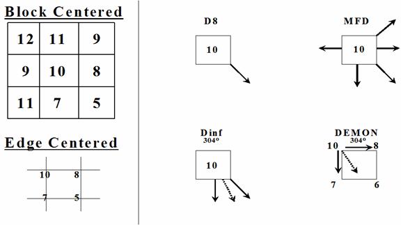
Figure 7. Schematic of the DEM pixel aspect computation and flow angle mapping performed by the D8, MFD, Dinf, and DEMON algorithms. Values on the left signify elevation. Solid arrows point in the direction that flow is mapped, and dotted lines correspond with the degree value above the pixel and indicate the pixel aspect for DEMON and Dinf. The distinctions between a block- and edge-centered DEM is illustrated (Endreny and Wood 2001)
2.6 Stream Channel Determination by Flow Accumulation
Once it is determined how water flows across a landscape, a flow accumulation value can be assigned to each cell showing how many cells are upstream from it. This simulates water as it accumulates going down hill to a stream channel. A user-determined accumulation cell threshold value identifies those cells that have concentrated flow and those cells that do not have concentrated flow. This threshold value defines the catchment size required for flow to become a stream channel.
Montgomery and Dietrich (1992) found that landscape dissection into distinct valleys is limited by a threshold of channelization that sets a finite scale to the landscape. This threshold determines the number of sub-basins that exist in the model. A small threshold results in a large number of small basins whereas a large threshold results in a small number of large basins. The threshold is equal to the hillslope length / accumulation that is just shorter than that necessary to support a channel head (Montgomery and Dietrich 1992). A threshold-based approach is most appropriate for modeling channel head locations over shorter, geomorphic time scales (e.g. 102-103 years) than modeling valley development (e.g. 104-106 years) (Montgomery and E. Foufoula-Georgiou 1993).
2.7 Generation of Flow Direction Networks
Many programs were used to implement the different flow direction models on a LiDAR DEM. SAGA (System for Automated Geoscientific Analyses) was the main interface used while ArcMap, TauDEM (Terrain Analysis Using Digital Elevation Models), and TAS (Terrain Analysis System) were used to verify that SAGA was performing the flow direction models properly (Appendix F). The reason that SAGA was used instead of other programs was its ability to store grid files in memory. Memory storage allowed the data to be compressed saving computer memory to permit more demanding tasks such as computing flow direction algorithms. The LiDAR DEM had to be broken up into individual sub-basins for the other programs to use the data. Because of the computational demand of DEMON, the 2-m LiDAR DEM had to be divided into the basin specific for the study site for SAGA to utilize the dataset.
2.8 Current Hydro Layer Evaluation
Evaluation of the
2.9 Field Measurements
Field locations
were sampled to test the accuracy of the current
Table 3. Stream parameters identified and collected in the field. The information was logged together with GPS coordinates.
Table 4. Fish presence or absence, % gradient and fish barrier type was logged with each stream feature type.
Field planning was
done by using LiDAR streams with the DNR hydro layer to locate stream features
in the field. The above values were
then determined and logged using a Trimble ProXRS
3. RESULTS
3.1 Flow Direction Comparison
The D8, Dinf, MFD, and DEMON predicted stream channel locations differently. The major difference in stream channel determination was in hillslope interpretation. Differences between D8 and DEMON decreased as resolution increased. From visually inspecting Figure 8, a 1:1 relation between D8 and DEMON at the 2-m resolution was shown using regression correlation, when a stream is defined as a 5-ha (13.2 (ln ft2)) basin. The models do not begin to correlate until 30.4-ha (15.0 (ln ft2)) at the 10-m USGS resolution from Figure 9. As resolution increased, the spread of the points in those figures becomes more confined to the lower left corner indicating the correlation between D8 and DEMON flow direction models. Table 5 summarizes the relationship between D8 and DEMON algorithms at various resolutions. No correlation can be determined with any combination of the other flow direction models with respect to increased resolution (Appendix G). APPENDIX G provides the plots of catchment area at all resolutions with the flow direction models used.
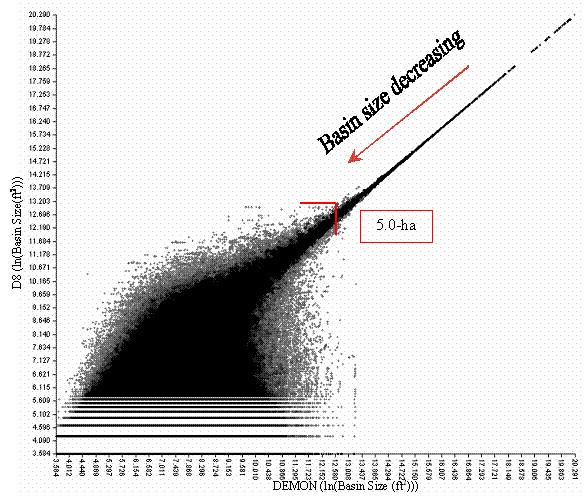
Figure 8. Cell plot of entire catchment area for a 2-m LiDAR DEM at the study site (Natural Log Values). D8 and DEMON correlate well above a threshold of approximately 5-ha as shown with the red mark. Below the 5-ha mark, differences are shown by the scatter.
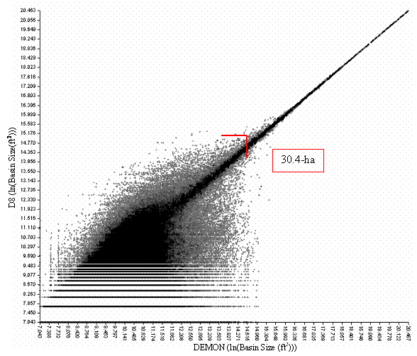
Figure 9. Cell plot of entire catchment area for the 10-m USGS at the study site (Natural Log Values). D8 and DEMON do correlate although not until a catchment area of approximately 30-ha is acceded as shown with the red mark. Below the 30-ha mark, differences are shown by the scatter.
Table 5. Relation between D8 and DEMON algorithms at various resolutions. As resolution is decreased, the correlation between D8 and DEMON becomes less. Basin size values determined by visually inspecting the plot of catchment area figures.

Using LiDAR datasets, D8 determines stream networks as well as DEMON. Endreny and Wood (2003) gave 2D-Lea (a building block in DEMON) the highest ranking in accuracy in comparison to any stream model that was used in their study. The data suggested that increased DEM resolution decreased the need for sophisticated models, reducing processing times required by complex models for high-resolution DEM’s. Since D8 is the most commonly used model and simplest to implement, computational time in computing stream networks is reduced in comparison to DEMON.
When comparing a LiDAR derived 10-m DEM with a USGS 10-m DEM, D8 stream channels with a catchment size of about 12-ha and greater somewhat converge between the two DEM’s (Figure 10). When catchments are less than 12-ha, no convergence existed. Since a USGS 10-m DEM contained topographic errors in regard to stream channel location, streams from the LiDAR and USGS were categorized as identical if they were less than 90-m apart to decrease error between the two datasets. This caused differences to decrease significantly between the two stream networks (Appeddix H). These differences occur in Strahler order 1,2 and 3 streams. The area in the lower middle of Figure 10 corresponds with areas when that the 10-m USGS under predicted stream channels in comparison to the area to the left side of the figure which corresponds to areas of under prediction of the LiDAR 10-m.
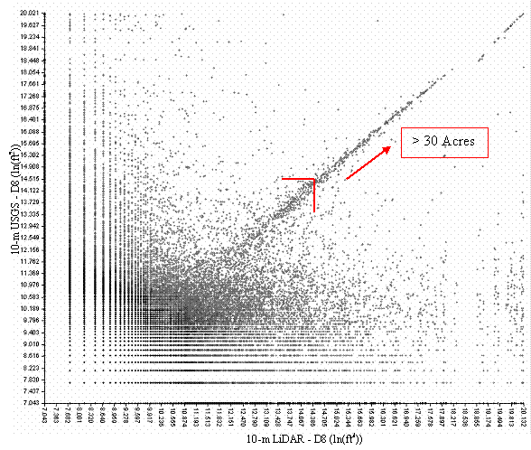
Figure 10. The D8 flow algorithm applied to the USGS and LiDAR Generated 10-m DEM. Illustrates that stream channels with a catchment size of about 12-ha and greater somewhat converge between the two DEM’s with regards to D8. When catchments are less than 12-ha, differences in stream channel location are shown by the scatter.
3.2 Resolution Effects on Flow Direction
As the DEM resolution increased, D8 model sensitivity also increased. At the 2-m resolution, a road crossing a stream is seen as a dam therefore routing the stream onto the road (Figure 11). The road influence alters stream location and extent. To correct this problem, known culvert locations, stream or ditch culverts at the study site were used to make the stream continue under the road. The LiDAR DEM was lowered in elevation at the culvert locations to cause the stream channels to flow to the culverts and away from the road. Culvert data causes the streams to flow to the main channel thereby minimizing road effects (Figure 12) (Schiess and Tyrall, 2003).
Decreasing the LiDAR-DEM resolution to 6-m removed the road effect and placed streams in a more realistic location than the 2-m uncorrected. At 6-m resolution, the stream models could not identify roads or the ditches associated with the roads. As the LiDAR-DEM resolution decreased, road influence decreased. Stream channels, for the most part, followed the corrected 2-m stream network (Figure 13). The advantage of the 6-m LiDAR-DEM was that it provided a significantly improved stream network compared to the 10-m USGS DEM and removed the need for culvert data.
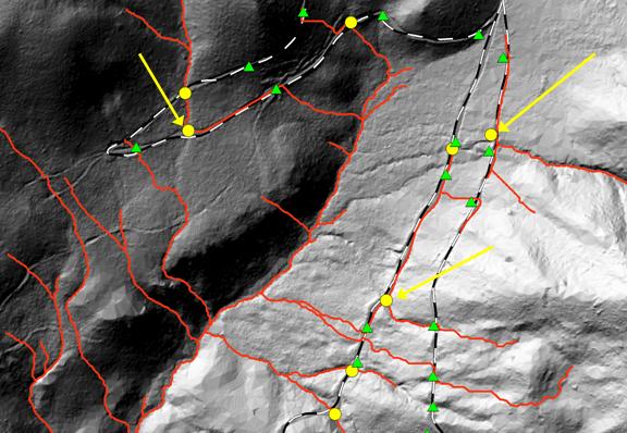
Figure 11. Streams generated from the 2-m LiDAR-DEM, in red, without using culvert correction. Stream culverts are circled, ditch culverts are triangles. At the 2-m resolution, the models defined some roads as stream channels bypassing the stream culverts (arrows).
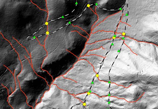
Figure 12. Streams generated from the 2-m LiDAR-DEM using culvert locations. Stream culverts are circled, ditch culverts are triangles. Culvert data causes the streams to flow downslope of the culvert allowing the stream to travel to the main channel more accurately.
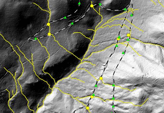
Figure 13. At 6-m resolution, the stream models did not route streams along roads and ditches. Removing the road effect placed streams in a reasonable location.
3.3 Assessing the Current Hydro Layer
Of the streams
that the WA
Very few of the
streams typed as 5 were dry and most were perennial. Figure 14 illustrates field verified
perennial streams identified using 6-m LiDAR DEM versus what the
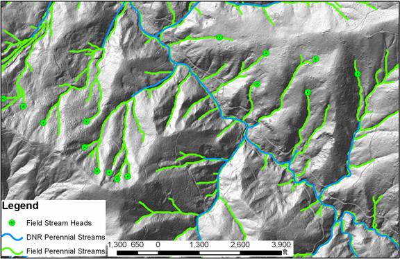
Figure 14. Field
verified perennial streams using LiDAR in green vs. what the
Table 6. Differences in perennial stream length between DNR hydro layer and the LiDAR stream network derived from 6-m LiDAR DEM.

*Uniform 30-m buffer for both datasets for Perennial flow
3.4 Determining Perennial Streams
Given the soils
geology and topography of the
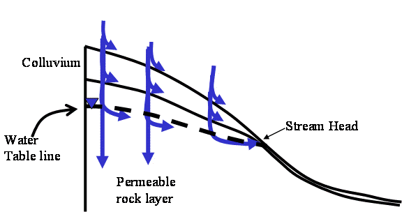
Figure 15. Stream head defined by the landscape. Perennial flow begins when ground water surfaced to form a stream head
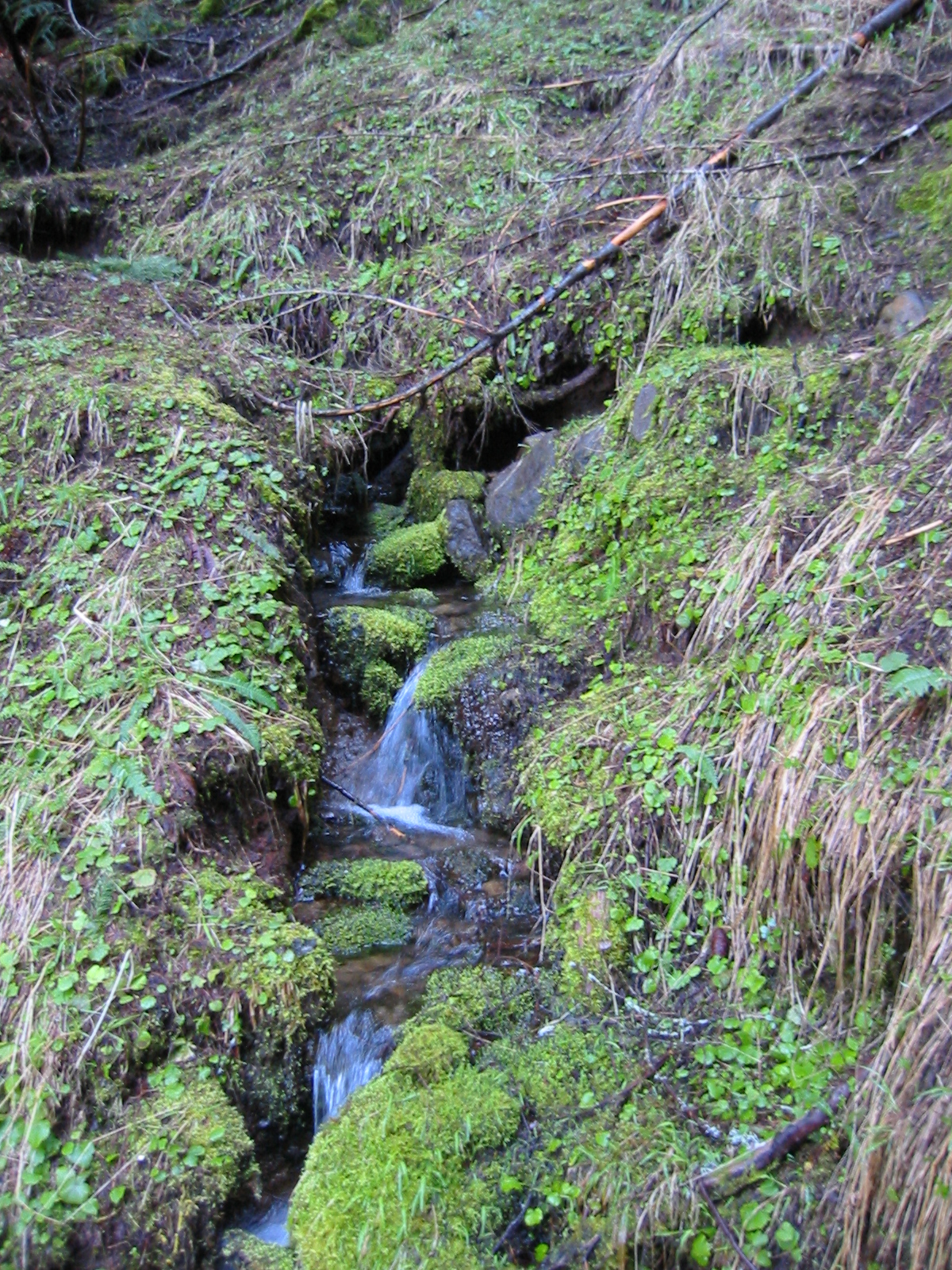
Figure 16. Spring identified as a stream head in the field.
In the field, 61
stream heads were located within the Mineral Creek,
53 heads were selected at random within the study site to be used to create a model to predict perennial initiation points (PIP).
Table 7. Sub-Basins used in perennial head identification with the number of stream heads visited in the field.
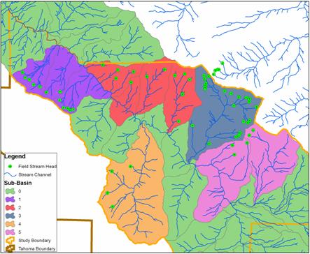
Figure 17. Stream heads in green within the study site. Stream channel generated from the 6-m LiDAR-DEM.
The final Linear Regression model for PIP used fewer variables than expected. The final model selected Basin Size using D8, Percent Slope, and Precipitation. Downstream gradient, forest density, elevation, and site class could not be used to create the equation for determining the probability of stream head locations based on a 0.05 significance level. Table 8 summarizes the variables uses for the regression. The Hosmer-Lemeshow chi-square statistic for this model was 10.262 and the -2 Log likelihood statistic was 80.130. Self-classification accuracies for this model were 77.4% for perennial flow and 88.7% for non-perennial flow. APPENDIX I provides further statistics regarding regression.
Table 8. Summary of the final logistic regression model.
|
Coefficients |
Estimate |
Standard Error |
Signifi- cance |
Exp(B) |
95.0% C.I. for Exp(B) | |
|
Lower |
Upper | |||||
|
Log10(Basin Size) |
7.235 |
1.425 |
0.000 |
1386.737 |
84.879 |
22656.314 |
|
Precipitation |
0.477 |
0.184 |
0.010 |
1.612 |
1.123 |
2.313 |
|
% Slope |
0.096 |
0.040 |
0.016 |
1.101 |
1.018 |
1.191 |
|
Constant |
-45.172 |
16.050 |
0.005 |
0.000 |
|
|
Using a model based on basin size alone for predicting perennial stream channels would be less accurate than the above model. The Hosmer-Lemeshow chi-square statistic for basin size model was 8.864 and the -2 Log likelihood statistic was 91.840. Self-classification accuracies for the basin size model were 77.4% for perennial flow and 84.9% for non-perennial flow. Overall, the average basin size for perennial flow for this model is 1.28-ha (3.16 acres).
Both models can
over estimate the extent of perennial stream channels by placing flow upstream
of the PIP. Using the conservative
approach described in the PIP Model section it has the potential to under
predict perennial flow. Using
average basin size determined from the field data, the average value is 2.2-ha
(5.44 acres). This average over and
under predicts perennial flow.
Since the Washington State Register defines contributing basin area as at
least 21-ha (52 acres), all models and approaches would significantly correct
The model in Table 8 was run at 4 different resolutions, 2-m, 6-m, 10-m LiDAR and a 10-m USGS DEM. Figure 18 illustrates the change in distance between modeled stream head location and field-verified stream head location for different DEM resolutions. This indicates that at all LiDAR resolutions, the error is relatively the same. The 10-m USGS DEM average distance and spread are higher than the LiDAR. This confirms that LiDAR improves upon modeling stream heads more accurately than a 10-m USGS DEM. The reasoning for high distances in the figure is due to the model not predicting a stream where the field verified stream head was located.
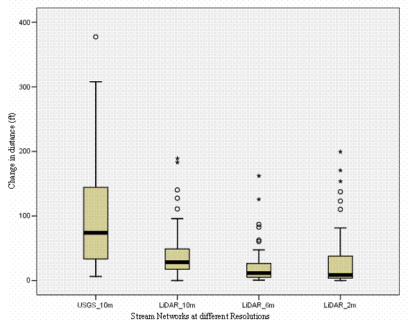
Figure 18. The distance error between modeled stream head location and field-verified stream head location at a given resolution. This indicates that at all LiDAR resolutions, the error is relatively the same. The 10-m USGS DEM average distance and spread are significantly higher than the LiDAR.
The PIP Model was tested on the various flow direction techniques listed in the “Flow Direction Methods Utilized” section to test which flow direction algorithm worked best in locating perennial flow. Because of the differences in the MFD and Dinf from D8, a separate bilinear regression model was created but none of the variables were significant based on a 0.05 significance level. The regression model in Table 8 was then used on the various algorithms on a 6-m LiDAR DEM to see the errors in predicted stream head locations. DEMON and D8 stream heads correlated in the difference in distance from the field-verified stream heads. Dinf and MFD increased in the difference in distance from field stream heads when compared to D8 (Figure 19). Finding a way to develop a bilinear regression model for Dinf and MFD would reduce the data error illustrated below.
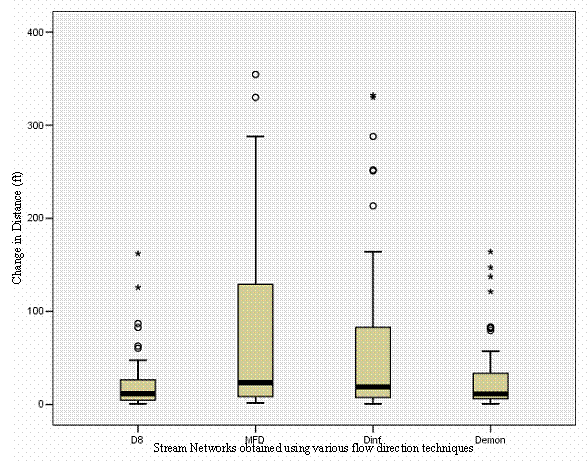
Figure 19. The distance error between field-verified stream heads and various flow direction modeled streams. DEMON and D8 correlated in error while Dinf and MFD significantly increased in error.
3.5 Determining Fish Stream Habitat
The CMER Model and Gradient Model estimated fish extent differently. CMER Model used basin area, downstream gradient, elevation, and precipitation, while the Gradient Model uses only downstream gradient. With field verification, the Gradient Model located fish barriers providing accurate fish habitat maps. The CMER Model tended to place potential fish waters well upstream of waterfalls and culvert barriers. Overall, the Gradient Model predicted fish extent closer to the main channel than the CMER method.
Figure 20 displays
a longitudinal profile of a selected creek generated by a LiDAR DEM. The red zones indicate field verified
waterfalls and culvert/road locations that the Gradient Model identified. These waterfalls can range from 1 to 6+
meters tall. If trout were able to
pass these barriers, the CMER Model would be correct in its estimation. Figure 21 shows the predicted fish
habitat estimated by the Gradient Model.
The CMER Model and
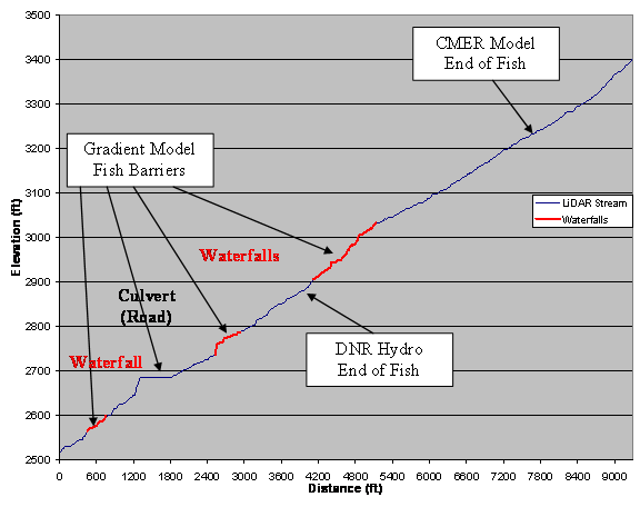
Figure 20. Longitudinal Profile of a selected creek. (Distance from main channel) The red zones indicate field verified waterfalls that the Gradient Model identified as well as culvert/road locations.
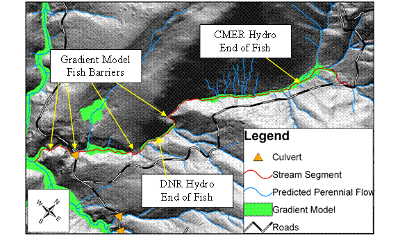
Figure 21. Stream Channel used (red) from Figure
20. This shows the predicted fish
habitat in green estimated by the Gradient Model. The CMER Model and
The CMER Model and
the
Table 9. Predicted Fish-Bearing Streams within the Study Site using different techniques.
The LiDAR DEM modeled fish barriers more accurately than a 10-m USGS DEM (Figure 20). At times, the USGS dataset resulted in incorrect locations for major waterfalls. In many cases, major waterfalls were not identified at all. For the most part, the USGS DEM identified the larger streams at the study site as accurately as the LiDAR DEM. This makes sense considering how the USGS DEM was created. Large streams are visible from aerial photos allowing elevation readings to be fairly accurate.
3.6 Weaknesses and Shortcomings
Having a LiDAR DEM
dataset provides the ability to model stream channels with their respective
stream head location more accurately compared to using the standard 10-m USGS
DEM. LiDAR DEMs also allow for more
accurately locating potential fish barriers. Currently, less than 1/5 of
Current spatial information usually does not have the fine resolution of a LiDAR dataset. Soils surveys, geology, and site class information are at lower resolutions than LiDAR so trying to develop a model that uses those themes could be difficult. These datasets would need to be at a higher resolution to better match a LiDAR derived dataset. The lack of a high-resolution site class map may explain why site class could not be used in the perennial stream regression model.
The major limitation to the regression model used to predict perennial flow is that it is site specific. While it proved to be more accurate than the current datasets available, accuracy may decrease when applying the model to a variety of landscape types. Data collected on a larger, more diverse area would generate a model better able to model landscapes.
In the middle of Figure 21 just below the “CMER Hydro End of Fish” label, a series of stream channels were identified in blue. This is a misrepresentation of the landscape due to dense forest canopy. A dense canopy will limit the amount of laser ground returns causing a loss of resolution in specific locations. A way to correct this problem would be to conduct field surveys of the landscape at those locations.
4. Conclusion
When used with high-resolution DEMs, the most common and least sophisticated algorithm to locate stream channels based on flow, D8, proved to be sufficient when compared to more complicated and process demanding algorithms. The advantage of D8 is that most programs like ArcGIS come standard with this algorithm to locate stream networks. In generating stream data using LiDAR, a computer with a high-speed processor is not necessary.
Increasing surface topographic resolution allowed an increase in the precision of stream channel modeling. Since the LiDAR DEM that was used for this project was at a 2-m resolution, decreasing the resolution of the LiDAR did not alter the ability to model locations of stream channels. The resolution at 2-m proved sensitive for the models used requiring a culvert dataset to alter stream flow off the road networks. Decreasing resolution to 6-m eliminates road effect errors. Relying on the resolution of a 10-m USGS DEM proved inadequate in modeling head water streams. High-resolution DEMs are necessary to accurately model stream networks.
As shown, a LiDAR DEM is a great source for generating hydrologic data by identifying probable perennial stream channels and locating fish barriers along a given stream. The ability to accurately model headwater streams and identify fish-bearing streams allows stream buffer zones to be in their topographically correct location. In turn it will allow for better planning at both the strategic (sustainable harvest volume calculations) and tactical or map scale level (forest operations planning at the watershed level) rather than having to rely on time-consuming field reconnaissance.
REFERENCES
Conrad, R.H., B.
Fransen, S. Duke, M. Liermann, and
Costa-Cabral, M. C. and S. J. Burges. 1994. Digital elevation model networks (DEMON): A model of flow over hillslopes for computation of contributing and dispersal areas. Water Resources Research, 30, 6, 1681-1692
Daly, C., C. Taylor,
and G. Taylor. 1988. 1961-1990 Mean Monthly Precipitation Maps for the
Conterminous
Daly, C., C. Taylor,
and G. Taylor. 2000. 1971-2000 Mean Monthly Precipitation Maps for the
Conterminous
Damian, F. 2001.
Improving cross drain culvert spacing with
Endreny, T. A., and Wood, E. F. 2003. Maximizing spatial congruence of observed and DEM-delineated overland flow networks. Int. J. Geographical Information Science. Vol. 17, No. 7, February 2003, pp. 699-713
Endreny, T. A., and Wood, E. F. 2001. Representing elevation uncertainty in runoff modeling and flowpath mapping. Hydrologic Processes. 15, 2223-2236 (2001)
Haugerud, R.A., and D. J. Harding. 2001. Some algorithms for virtual deforestation (VDF) of LiDAR topographic survey data. International Archives of Photogrammetry and Remote Sensing. XXXIV-3/W4, p. 211–217. duff.geology.washington.edu/data/raster/LiDAR/vdf4.pdf (March 2003).
Jenson S. K. and J. O. Domingue. 1988. Extracting topographic structure from digital elevation data for geographic information systems analysis. Photogrammetric Engineering and Remote Sensing. Vol. 54, No. 11, pp. 1593-1600
Latterell, J. J., R.
J. Naiman, B. R. Fransen, and P. A. Bisson. 2003. Physical constraints on trout
(Oncorhynchus spp.) distribution in the
Luijten, J, 2000.
Dynamic hydrological modeling using ArcView
Montgomery, D. R. and W. E. Dietrich. 1992. Channel initiation and the problem of landscape scale. Science, 255: 826-830.
Moore,
Moore,
O’Callaghan, J. F., and D. M. Mark. 1984. The extraction of drainage networks from digital elevation data. Comput. Vision Graphics Image Processing, 28, 323-344
Oladi, D. 2001.
Developing a forest growth monitoring model using thematic mappery imagery.
Proc. ACRS 2001 - 22nd Asian Conference on Remote Sensing, 5-9 November 2001,
Pan, F., C. D. Peters-Lidard, M. J. Sale, A. W. King. 2004. A comparison of geographical information systems-based algorithms for computing the TOPMODEL topographic index. Water Resource Research, 40.
Quinn, P. F., K. J. Beven, P. Chevallier, and O. Planchon. 1991. The prediction of hillslope flow paths for distributed hydrological modeling using digital terrain models. Hydrol. Processes, 5, 59-80
Renslow, M. S. 2001. Development of a bare ground DEM and canopy layer in NW forestlands using high performance LiDAR. Int'l User Conf., ESRI.
Schiess, P. and A.
Mouton, 2005. North Fork Mineral Creek access and transportation strategy.
Techn. Report,
Schiess, P. and J.
Tyrall, 2002.
Schiess, P. and J.
Tryrall, 2003. Developing a road system strategy for the
Schiess, P. and Krogstad, F. 2003. LiDAR-based topographic maps improve agreement between office-designed and field-verified road locations. Proceedings of the 26th Annual Meeting of the Council on Forest Engineering,, Bar Harbor, Maine, USA, 7-10 September, 2003
Shamayleh,
H,. and A. Khattak. 2003. Utilization of LiDAR technology for highway inventory.
Mid-Continent Transportation Research Symposium,
Soil Survey
Staff. 1998. Official series description – Bellicum, Cattcreek, and Cotteral
series. Natural Resources Conservation
Strahler, A.N. 1957.
Quantitative analysis of watershed geomorphology. Transactions of the American
Geophysical
Tarboton,
D. G., R. L. Bras, and
Tarboton, D. G. 1997. A new method for the determination of flow direction and upslope areas in grid digital elevation models. Water Resour. Res., 33(2), 309-319
Tarboton,
D. G. 2003. Terrain analysis using digital elevation models in hydrology. 23rd
ESRI International Users Conference,
Terrapin
Environmental. 2003. Water typing model gield validation study design approach
and procedures. Westside Water Type Model Validation Plan,
Wilson J.
P. and J. C. Gallant (editors). 2000. Terrain analysis: Principles and
Applications.
Wolock, D. M., and G. J. McCabe. 1995. Comparison of single and multiple flow direction algorithms for computing topographic parameters. Water Resour. Res., 31(5), 1315-1324
- Remotely Sensing
The main objectives are:
o To identify non-industrial tax parcels either taxed as forestland by the county assessor or that are completely within a forested area.
o To construct a spatially explicit GIS based dataset that identifies these parcels and their owners.
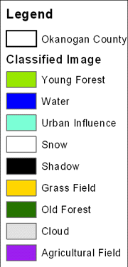
ERDAS Imagine 8.6 was used to read Landsat 7 images and run a rectification process to eliminate atmospheric effects that exist in all remotely sensed images. Using orthographically corrected aerial photos as ground truth data, forest land was identified as well as other land cover types such as urban, agriculture, water, snow and clouds. ERDAS was then used to run a supervised classification of the land cover types identified using the ortho photos. The classified land cover classes were then overlaid on the county parcel data to determine which parcel were forested. Using ArcGIS 8.3, the classified Landsat data and the parcels were intersected to produce a dataset showing the proportion of each parcel that is forested.
Landsat 7 Classification Example
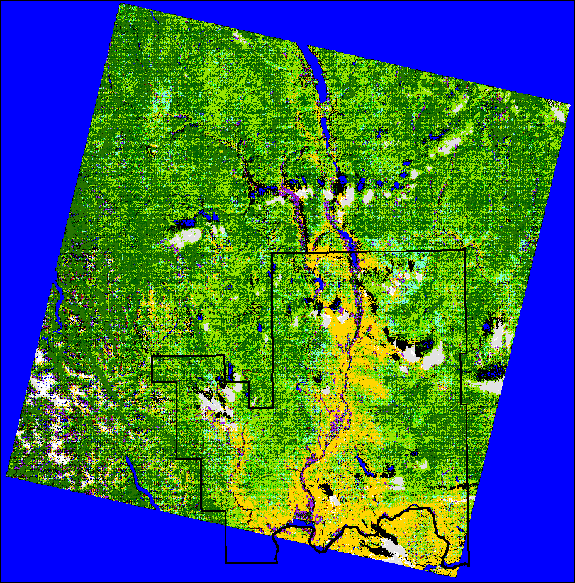
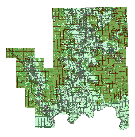
The results showed the non-forested parcels are in and around the urban areas. The result of the GIS intersection between the parcel and the forests indicated how many acres of a parcel are forested, the percentage of forest based on the total area of the parcel, and if trees exist in the parcel. With this information and other fields in the table of the intersection, we can identify whether or not a parcel may be non-industrial private forestland.
REFERENCES
Jensen, John R., "Digital Techniques of Remote Sensing", USC Geography, Feb. 2003,
http://www.cla.sc.edu/geog/rslab/751/
NASA "Landsat 7 Science Data User Handbook, Chapter 11 Data Products", April 2004,
http://ltpwww.gsfc.nasa.gov/IAS/handbook/handbook_htmls/chapter11/chapter11.html
Emch, Michael E., "Imagine Exercise 8: Spatial, radiometric, and spectral enhancement", April 2004,
http://web.pdx.edu/~emch/rs/EX8rs.html